10 gruesome images of adversarial networks fighting to the death

Introduction
Adversarial autoencoders have been used to synthesize images, so I thought they might be employed to synthesize sound as well. One obvious difference is that images are static in time, while sound could go on forever, with each new bit of sound depending on all previous sound. This is a difficult property of sound, and to simplify it, I think autoencoders might initially provide a hybrid approach somewhere between granular synthesis and deep learning. My idea is that an auto encoder might be able to generate short windows (grains) of audio that would behave computationally like images, and that could later be assembled via granular synthesis. There might later be a separate machine learning thing that would tell us in what order to assemble the windows (more on this anon).The code described in this post is in the Ambisynth Private Repository
Autoencoders

Figure 1: Schematic of an autoencoder. A window of audio samples goes in the top, flows through a bottleneck, and hopefully what comes out the bottom is more or less identical to the original window of audio
An autoencoder, such as seen in Figure 1, is a neural network with a bottleneck. The part above the bottleneck is the encoder, and below is the decoder. The encoder takes a window of audio samples as input, and outputs codes at the bottleneck. The decoder takes those codes and outputs audio. The whole thing is trained to try to make the output match the input. Later, after training, when we want to synthesize a window of audio, we should be able throw away the encoder and put codes directly into the decoder. Given the right codes, the decoder should output audio that resembles the training data.
Autoencoders of this type are relatively easy to train. I used a window size of 1002 samples (22 milliseconds at 22050 Hz), a code size of 10 numbers, and one 1002-unit hidden layer in each of the encoder and decoder. After training for only a few minutes on Lakeside from DCASE 2016, the output matched the input relatively well. Examples are shown in Figure 2.

Figure 2: Windows of audio. In orange are the original waveforms taken out of the lakeside recordings (input to the autoencoder), and in blue are the autoencoded versions (output of the autoencoder).
These results aren't bad, and could undoubtedly be improved with more training. The problem is that we can't use this to synthesize more audio, because we don't know what the codes are. In particular, the codes might not be compact. Imagine that the codes are just a single real number. Non-compactness means that, for example, a code value of 0.132489 might output a nice window of audio, and a code value of 5793270345.45987 might also output a nice window of audio, but everything in-between might output garbage.
Adversarial Autoencoders
We can use an adversarial autoencoder to force the encoder to output to be compact, and to lie in some range that we specify. A diagram of an adversarial autoencoder is shown in Figure 3.
Figure 3: Schematic of an adversarial autoencoder. It is like a regular autoencoder, but has an additional adversarial network (the Adjudicator) that forces the codes output by the encoder to be in the desired range.
More details about how this works is in other blog posts, like this one and this one, so I won't go into too much detail. I will just point out that the encoder is in an adversarial relationship with the adjudicator, and the adjudicator is adversarial about the codes, not about the audio. During training, at each step, the encoder is trained alternatively with the decoder (to try to produce good audio) and the adjudicator (to try to produce good codes).
Adversarial Autoencoder Results
So I built a network where the encoder, adjudicator, and decoder all have 2 hidden layers with 1000 units each. The window size is still 1002 and the code size is still 10. I trained this for about a day and a half on a cpu-only machine. For posterity, the loss function of the networks are shown in Figure 4
Figure 4: Loss functions of the adversarial autoencoder from 0 to 1000 cycles, 15k to 16k cycles, and 29k to 30k cycles.
For now, the main take-away is that from the plot on top, I convinced myself that training was essentially finished after 30k training cycles, so I stoped training it to sample its performance.
Codes
I had trained the network in such a way that the codes should follow a Gaussian distribution with mean 0 and standard deviation of 5. To check if this worked, I fed many windows of audio into the encoder and plotted the distribution of the codes that came out. The result is in Figure 5, and closely matches the desired distribution.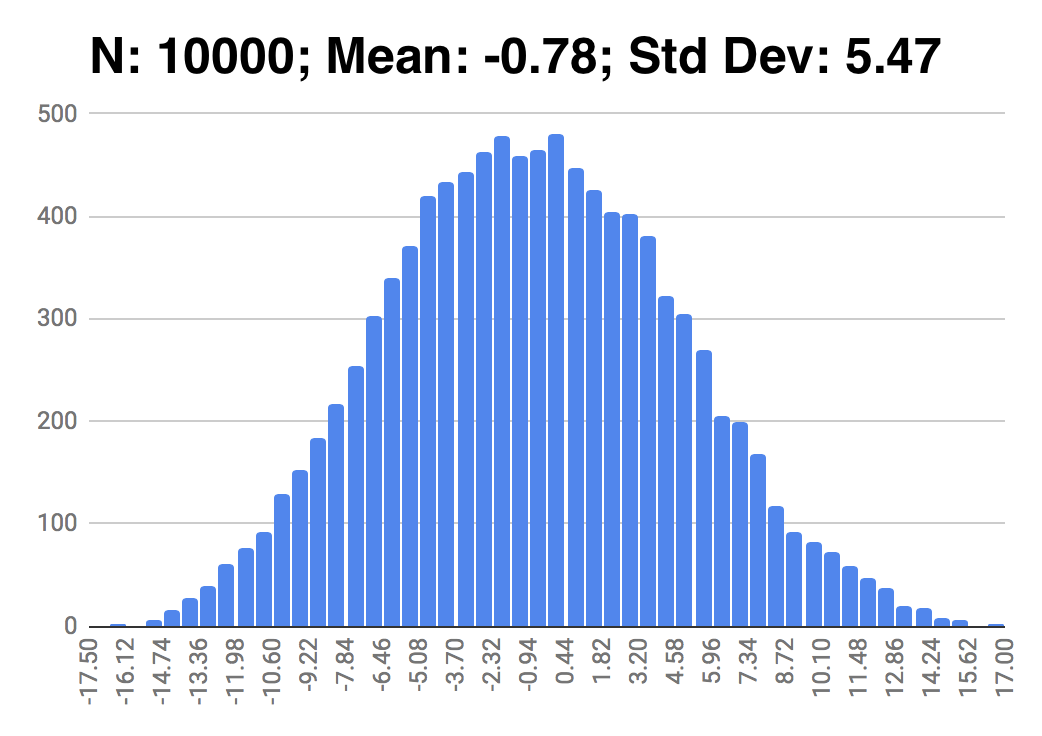
Figure 5: Distribution of code values after training for 30k cycles, closely matching the desired distribution.
Now that we know where the codes are, we should be able to navigate the code space. We know that the codes lie mostly between about plus or minus 10, and moreover, similar codes should cause the decoder output similar sounds. This might mean that all ocean-wave-like sounds are grouped together and all wind-like sounds are grouped together. This is depicted in Figure 6

Figure 6: Hypothetical code space. Codes here consist of 2 values, x and y. The codes in the lower-left quadrant will cause the decoder to output wind-sounds, the top-right will output wave sounds. A soundscape might be thought of as a path through this space over time, e.g. starting with wind, wandering though other sounds, and ending up with waves.
So, if we input a code, we should get out a window of audio that could be used as a grain in a granular synthesizer. Over time, we could navigate a path through the code space to produce different types of sounds. In the future, valid paths might be learned as a separate deep-learning procedure, for instance using Alex Graves's famous paper on learning pen-strokes in handwriting.
Audio Results
To check the audio results, I put some random windows of audio into the encoder and compared the input to the decoder output. The results are in Figure 7.
Figure 7: Input (orange) vs output (blue) of the autoencoder after trained for 30k training cycles.
Additionally, I took non-overlapping windows sequentially out of a 10-second audio file, encoded and decoded each window, and put the results into a new 10-second audio file. Of course I don't expect the output windows to adjoin nicely, but this should give some idea of the performance. The result is in Figure 8 and Example 1.

Figure 8: Bottom -- 10 seconds of mono audio from DCASE 2016 Lakeside. Top -- Synthesized version of the same audio file, made by sequentially auto-encoding the original audio file in 20 millisecond chunks. (These waveforms can be heard in Example 1).
Example 1: Adversarial Autoencoder output. I sequentially took 22-millisecond non-overlapping windows out of a 10-second lakeside recording, ran each window through the autoencoder, and sequentially put the result back into a new audio file. Bottom is the original lakeside recording, and Top is the re-synthesized version.
From Example 1 and Figures 7 and 8, it can be seen that the autoencoder output does approximate its input, but also that the output is very noisy. A spectrum of a window of audio is seen in Figure 9, and shows that the noise at the encoder output appears to be white.

Figure 9: Spectrum of a grain of audio as input into (orange) and output from (blue) the autoencoder, showing the output noise to be evidently flat.
This should be relatively easy to filter out. I zeroed out the right 85 percent (gasp!) of the frequency bins. Results for some windows are shown in Figure 10.

Figure 10: Input (orange) and filtered output (blue) of autoencoder
Visually, these look relatively good. I'm afraid to hear what this sounds like, so I guess I'll just pack it up and call it a day. Good work, Mike.
... Ok, ok, I made a new audio file similar to Example 1, except that I took overlapping windows out of the original file, filtered each window, and applied a Blackman Window Function before putting it in the output audio file, overlapping the previous grains. I used 90 percent overlap. The result is in Example 2.
Example 2: Adversarial Autoencoder output. I sequentially took 22-millisecond overlapping windows out of a 10-second lakeside recording, ran each window through the autoencoder, filtered and applied a Blackman function to each, and sequentially put each window back into a new audio file.
Observations
Example 2 is difficult to interpret for a number of reasons. First let's acknowledge that it doesn't sound that great. One issue is that there was so much noise, and we filtered it so heavily that not much definition of any type remains. Anyway, if we are going to use such aggressive filtering, we could have just started with a lower sampling rate and greatly reduced the size and training time of the network to begin with, and gotten equivalent results. Moreover, there is a pitched buzzing sound present throughout -- this is a side effect of the granular synthesizer, and can be mitigated by varying the grain length and placement, so for now I'm not too worried about it. The most import observation is that I can't really tell whether or not this audio retained any properties of the original lakeside audio. That dataset is all basically filtered noise to begin with, and I can't tell how much of what we have here is desired versus undesired noise. I should probably repeat this experiment with something like speech or something with more definition.Reflections on the Results
For images, autoencoders are often used as denoisers, so why should our autoencoder be adding noise? My hypothesis is that it is because, for audio, the input could appear in any rotation. For images, say images of faces, the image would never be rotated so the ears appear at the middle and the nose, split in half, at the edges. The eyes are always roughly in the same place. If you average together many face images, you get a blurry face. With audio, a feature that appears on the left on one window could appear later on the right of another window. If you average together audio windows, you get naught. Any sample could take any value, so noise is sort of built in to the average, in a way.Spectral Autoencoder
The Fourier transform has the nice property that it is not local, so features on the left will always be on the left, regardless of where they appeared in the original audio. So I thought learning the spectra might be easier that learning the audio directly. To test this, I built a vanilla, non-adversarial autoencoder, such as is depicted in Figure 1, and used the DFT of each window instead of the raw audio samples. I used the (scaled) magnitude in the first half of the inputs and (scaled) phase in the last half of the inputs. From each phase I added or subtracted multiples of 2π radians from each phase such that no two consecutive phases differed by more than π/2. I trained it only for 3000 training cycles. This is not fully trained, but it was enough to convince me that it is not converging quickly enough to produce better results than using raw audio, especially considering that adversarial models seem to output more noise than non-adversarial models. Example output from this model is shown in Figure 11.
Figure 11: Example input (orange) and output (blue) from an autoencoder trained using the DFT of a window of audio instead of the raw audio. Top left shows the magnitude of the DFT, and top right shows the phase. Bottom shows the original audio waveform, and the reconstructed audio made by performing the inverse DFT on the autoencoder's output spectrum.
I think the main difficulty here is the phases. Perhaps more on that another day.


Comments
Post a Comment